In this post, I will walk through one of the most widely used methods in survival analysis: the Cox proportional hazards model.

Photo by Alexander Andrews on Unsplash
Before jumping into the Cox model, it is helpful to clarify how parametric, semi-parametric, and non-parametric survival models differ.
Parametric, Semi-Parametric, and Non-Parametric Models
According to Ravi Charan (Charan 2020), the models can be summarised as follows:
Non-parametric models make no assumption about the functional form of the hazard function, \(\lambda(t)\). A common example is the Kaplan-Meier estimator.
Parametric models assume a specific distribution for survival time, such as exponential, Weibull, log-normal, or log-logistic. This implies a specific shape for the hazard function.
Semi-parametric models sit between these two approaches. The Cox proportional hazards model does not require us to specify the shape of the baseline hazard function.
- Instead, the model focuses on estimating how covariates change the hazard relative to the baseline hazard.
Cox Proportional Hazards Model
What is the Cox proportional hazards model?
The Cox proportional hazards model is a semi-parametric survival model that estimates the relationship between covariates and the hazard of an event occurring.
The model can be written as follows (STHDA, n.d.):
\[h(t) = h_0(t) \times exp(b_1x_1 + b_2x_2 + ... + b_px_p) \]
where
\(t\) is the survival time
\(h(t)\) is the hazard function for an individual with covariates (\(x_1, x_2, ..., x_p\))
(\(b_1, b_2, ...., b_p\)) are coefficients that measure the effect of the covariates
\(h_0(t)\) is the baseline hazard, which represents the hazard when all covariates are at zero or at their reference levels
The key idea is that covariates multiply the baseline hazard. This allows us to estimate how several risk factors are associated with the event rate at the same time, without having to specify the exact shape of the baseline hazard over time.
How to interpret a Cox model
One of the key outputs from a Cox model is the hazard ratio, which is calculated as \(exp(coef)\).
The hazard ratio is a relative measure. It compares the hazard between two groups, or between two values of a numeric variable, while holding the other variables in the model constant.
Categorical variable
Hazard ratio = 1: no difference in hazard compared with the reference group
Hazard ratio > 1: higher hazard compared with the reference group
Hazard ratio < 1: lower hazard compared with the reference group
Numerical variable
For a numeric variable, the hazard ratio represents the multiplicative change in the hazard for a one-unit increase in that variable, holding the other variables constant.
For example, if the hazard ratio for age is 1.05, then a one-year increase in age is associated with a 5% higher hazard, all else being equal. This does not mean the probability of the event increases by exactly 5%; it means the instantaneous event rate is 5% higher at a given point in time.
Cox proportional hazards model vs. Kaplan-Meier survival curve

The Kaplan-Meier curve is useful for estimating and visualising survival probabilities over time, especially for a small number of groups. However, it has some practical limitations:
It does not directly model several explanatory variables at once.
Numeric variables often need to be grouped before plotting, otherwise each unique value may effectively behave like a separate group.
It is mainly descriptive, whereas the Cox model allows us to estimate the association between covariates and the hazard of the event.
These issues can be addressed with the Cox proportional hazards model. However, the Cox model also has its own assumptions, especially the proportional hazards assumption, which we should check before relying on the results.
Concordance Index
Before moving to the demonstration, it is useful to introduce one common performance metric for survival models: the concordance index, or C-index.
The C-index measures how well the model ranks subjects by risk. More specifically, it can be interpreted as the fraction of comparable pairs whose predicted risks are correctly ordered with respect to their observed event times (Raykar et al., n.d.).
Below is a chart showing how the concordance index is calculated:
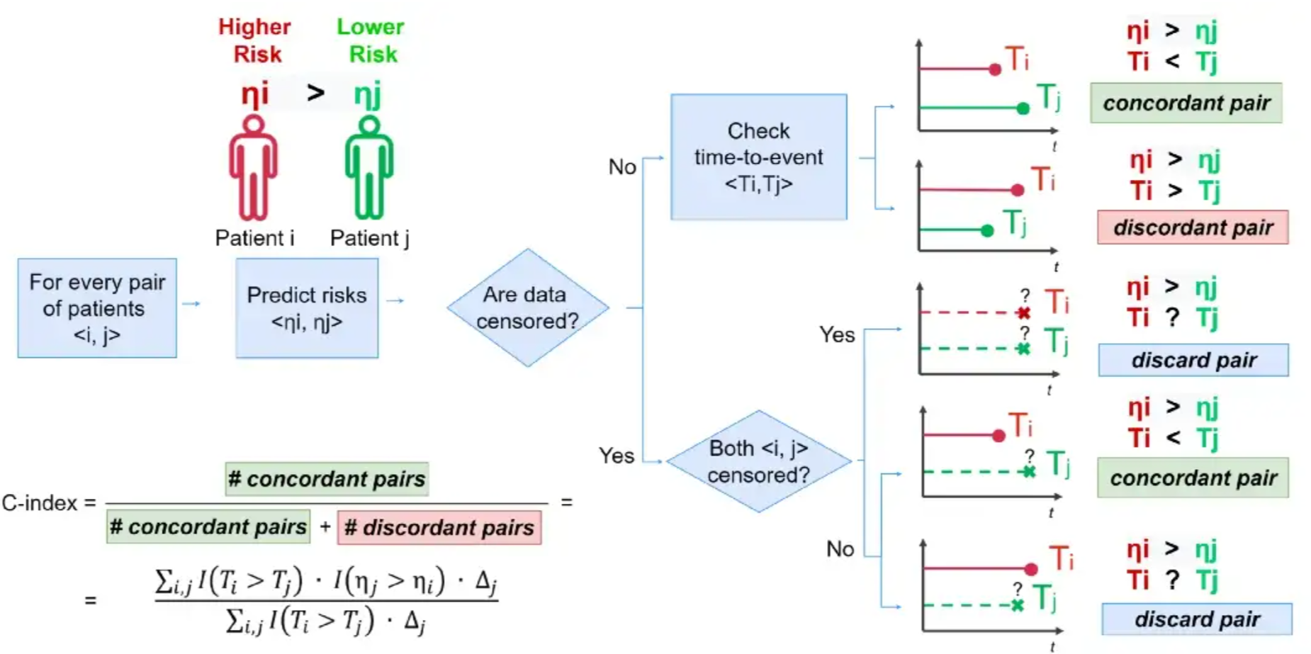
Taken from “How to Evaluate Survival Analysis Models” post by Nicolo Cosimo Albanese
The interpretation can be summarised as follows:
C = 1: perfect concordance between predicted risk and event time.
C = 0.5: no better than random ranking.
C = 0: perfect anti-concordance between predicted risk and event time.
In practice, the C-index should not be the only metric used to assess a survival model. It measures ranking performance, but it does not tell us whether the model is well calibrated, whether the proportional hazards assumption is reasonable, or whether the model generalises to new data.
Demonstration
In this demonstration, I will use this bank churn dataset from Kaggle.
One important caveat: this dataset is not a perfect survival dataset. The variable tenure is used as the time variable and exited is used as the event indicator. Customers who have not exited are treated as right-censored at their current tenure. This is a useful way to demonstrate the Cox model mechanics, but in a real churn analysis we would want a proper customer history with start dates, event dates, observation windows, and censoring rules.
Setup the environment
In this demonstration, I will use the coxph function from the survival package to build the Cox proportional hazards model.
I will use functions from the survminer package to visualise the results.
First, I will load the necessary packages into the environment.
pacman::p_load(tidyverse, lubridate, janitor, survival, survminer, scales)Import data
Next, I will import the dataset into the environment.
I will also clean the column names, drop columns that are not useful for modelling, and transform selected columns to the right format.
df <- read_csv("https://raw.githubusercontent.com/jasperlok/my-blog/master/_posts/2022-09-10-kaplan-meier/data/Churn_Modelling.csv") %>%
  clean_names() %>%
  select(-c(row_number, customer_id, surname)) %>%
  mutate(has_cr_card = factor(has_cr_card),
         is_active_member = factor(is_active_member),
         credit_score = credit_score/100,
         balance = balance/10000,
         estimated_salary = estimated_salary/10000) %>%
  filter(tenure > 0)
Note that I have scaled credit_score, balance, and estimated_salary. This makes the model output easier to interpret because the hazard ratios are no longer based on very small unit changes.
Build the Cox model
To build the Cox model, I will use the coxph function from the survival package.
cox_model <- coxph(Surv(tenure, exited) ~ .,
                   data = df,
                   x = TRUE,
                   y = TRUE)
We can call the fitted model to see the model result.
cox_modelCall:
coxph(formula = Surv(tenure, exited) ~ ., data = df, x = TRUE,
y = TRUE)
coef exp(coef) se(coef) z p
credit_score -0.048759 0.952410 0.023060 -2.114 0.0345
geographyGermany 0.488400 1.629706 0.055680 8.772 < 2e-16
geographySpain 0.034473 1.035074 0.062178 0.554 0.5793
genderMale -0.382557 0.682115 0.045836 -8.346 < 2e-16
age 0.048125 1.049302 0.001816 26.506 < 2e-16
balance 0.020393 1.020603 0.004495 4.537 5.7e-06
num_of_products -0.051172 0.950116 0.039461 -1.297 0.1947
has_cr_card1 -0.059315 0.942410 0.049585 -1.196 0.2316
is_active_member1 -0.755391 0.469827 0.048751 -15.495 < 2e-16
estimated_salary 0.001221 1.001222 0.003926 0.311 0.7558
Likelihood ratio test=1124 on 10 df, p=< 2.2e-16
n= 9587, number of events= 1942 The summary function provides more detailed information about the fitted model.
summary(cox_model)Call:
coxph(formula = Surv(tenure, exited) ~ ., data = df, x = TRUE,
y = TRUE)
n= 9587, number of events= 1942
coef exp(coef) se(coef) z Pr(>|z|)
credit_score -0.048759 0.952410 0.023060 -2.114 0.0345 *
geographyGermany 0.488400 1.629706 0.055680 8.772 < 2e-16 ***
geographySpain 0.034473 1.035074 0.062178 0.554 0.5793
genderMale -0.382557 0.682115 0.045836 -8.346 < 2e-16 ***
age 0.048125 1.049302 0.001816 26.506 < 2e-16 ***
balance 0.020393 1.020603 0.004495 4.537 5.7e-06 ***
num_of_products -0.051172 0.950116 0.039461 -1.297 0.1947
has_cr_card1 -0.059315 0.942410 0.049585 -1.196 0.2316
is_active_member1 -0.755391 0.469827 0.048751 -15.495 < 2e-16 ***
estimated_salary 0.001221 1.001222 0.003926 0.311 0.7558
---
Signif. codes: 0 '***' 0.001 '**' 0.01 '*' 0.05 '.' 0.1 ' ' 1
exp(coef) exp(-coef) lower .95 upper .95
credit_score 0.9524 1.0500 0.9103 0.9964
geographyGermany 1.6297 0.6136 1.4612 1.8176
geographySpain 1.0351 0.9661 0.9163 1.1692
genderMale 0.6821 1.4660 0.6235 0.7462
age 1.0493 0.9530 1.0456 1.0530
balance 1.0206 0.9798 1.0117 1.0296
num_of_products 0.9501 1.0525 0.8794 1.0265
has_cr_card1 0.9424 1.0611 0.8551 1.0386
is_active_member1 0.4698 2.1284 0.4270 0.5169
estimated_salary 1.0012 0.9988 0.9935 1.0090
Concordance= 0.72 (se = 0.006 )
Likelihood ratio test= 1124 on 10 df, p=<2e-16
Wald test = 1169 on 10 df, p=<2e-16
Score (logrank) test = 1211 on 10 df, p=<2e-16The hazard ratio is shown as exp(coef) in the output.
The three tests at the bottom of the results are overall significance tests for the model. The null hypothesis is:
\(H_0:\beta = 0\)
In other words, the null hypothesis is that the covariates have no association with the hazard. Since the p-values for all three tests are smaller than 0.05, we reject the null hypothesis and conclude that the model contains at least some useful predictors.
This does not mean every individual variable is important, nor does it prove causality. It means the model as a whole provides evidence of association between the covariates and churn hazard.
For more information on how to interpret the result, I find this post very helpful.
Alternatively, chapter 5 of the book Applied Survival Analysis Using R by Dirk F. Moore has a clear explanation of Cox proportional hazards as well.
Extract the results
The concordance result can be extracted using the following method:
cox_model$concordance["concordance"]concordance
0.7204698 Alternatively, we can extract the concordance index by passing the fitted model into the concordance function from the survival package.
concordance(cox_model)Call:
concordance.coxph(object = cox_model)
n= 9587
Concordance= 0.7205 se= 0.006461
concordant discordant tied.x tied.y tied.xy
7192433 2790544 0 193333 0 The full model has a C-index of approximately 0.72 in the rendered output, which suggests a reasonable ability to rank customers by relative churn risk. However, this is still an in-sample result. For a stronger analysis, we should evaluate the model on a validation or test set.
Check the proportional hazards assumption
Because the Cox model assumes proportional hazards, we should check whether the effect of each covariate is reasonably constant over time.
The cox.zph function tests the proportional hazards assumption using Schoenfeld residuals.
ph_test <- cox.zph(cox_model)

ph_test
chisq df p
credit_score 2.33e-01 1 0.629
geography 3.88e+00 2 0.144
gender 1.16e-01 1 0.733
age 1.34e+00 1 0.246
balance 4.27e+00 1 0.039
num_of_products 5.70e-01 1 0.450
has_cr_card 2.88e-04 1 0.986
is_active_member 1.84e+00 1 0.174
estimated_salary 1.07e+00 1 0.301
GLOBAL 1.29e+01 10 0.232ggcoxzph(ph_test)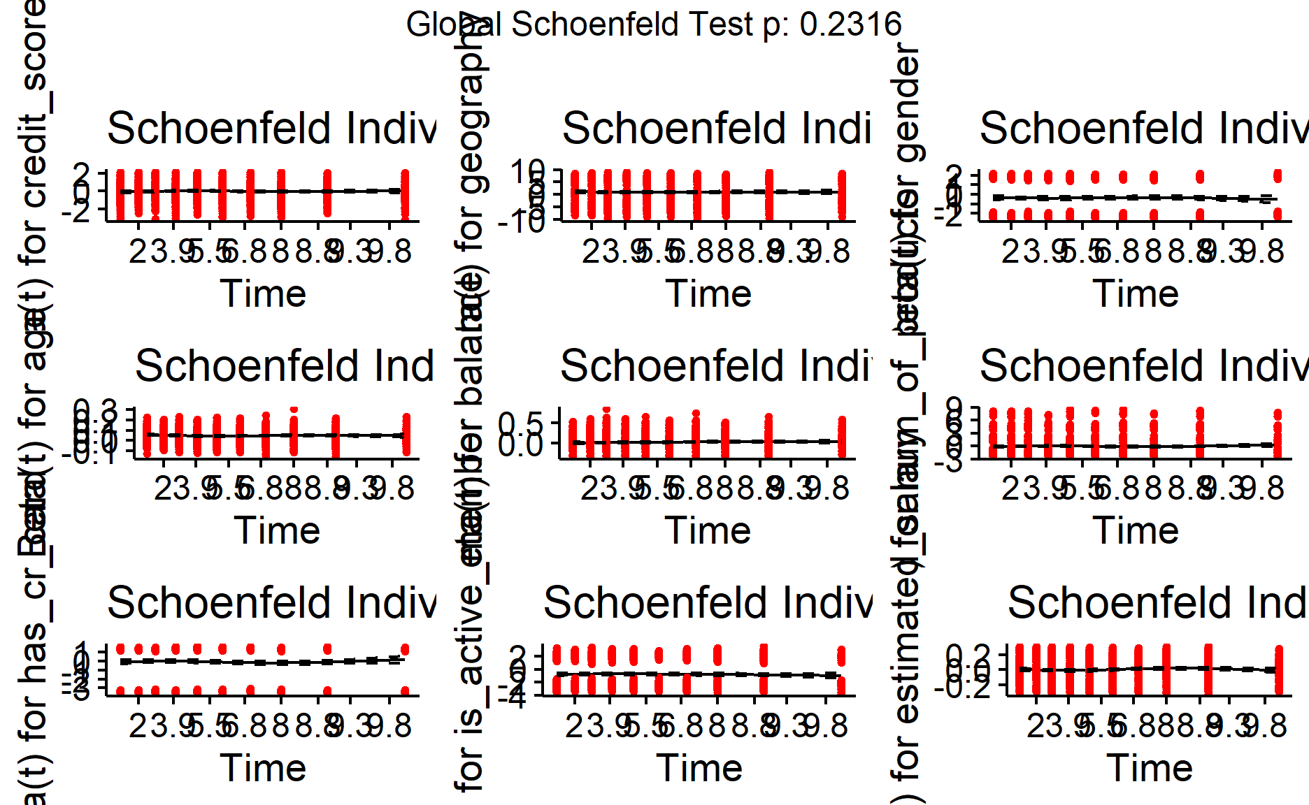
If the test suggests that a variable violates the proportional hazards assumption, we should not ignore it. Possible next steps include adding time-varying effects, stratifying by that variable, transforming variables, or using a different modelling approach.
Visualise the survival curve
After fitting a Cox model, it is possible to visualise the predicted survival proportion at each time point for a given covariate profile. The survfit() function estimates the survival curve from the fitted model. By default, it uses a typical covariate profile based on the covariate values in the data.
ggsurvplot(survfit(cox_model),
           data = df)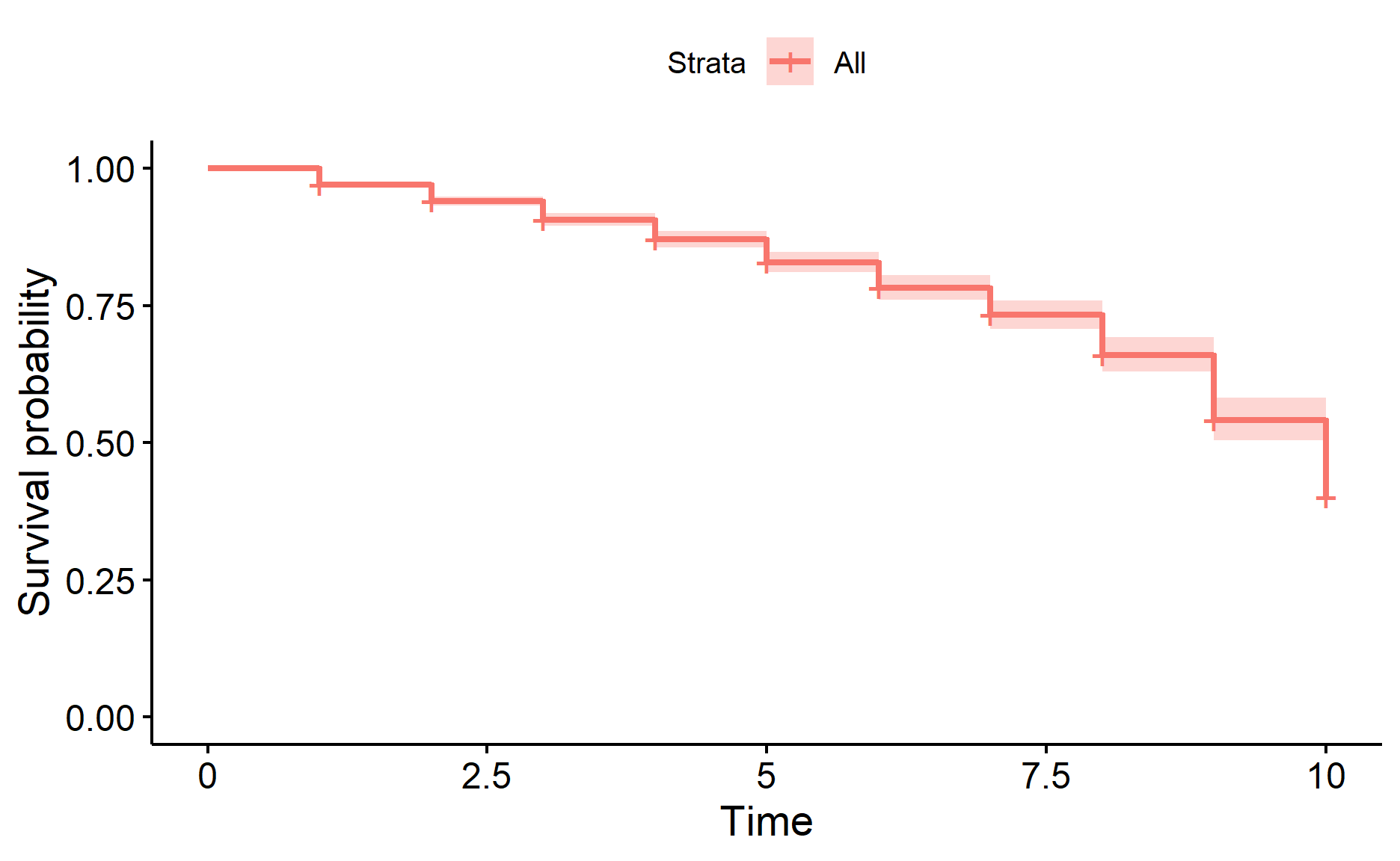
To plot the graph, we pass the fitted Cox model into the survfit function.
ggsurvplot also supports multiple survival curves.
To demonstrate this, I will split the dataset by gender.
Then, I will fit two Cox proportional hazards models based on each dataset.
survfit_male <-
  coxph(Surv(tenure, exited) ~ .,
        data = df_male)

survfit_female <-
  coxph(Surv(tenure, exited) ~ .,
        data = df_female)
Then, I will create a list before passing it into the ggsurvplot function.
surv_fit_list <-
  list("male" = survfit(survfit_male),
       "female" = survfit(survfit_female))

ggsurvplot(surv_fit_list,
           combine = TRUE,
           conf.int = TRUE,
           ylim = c(0.35, 1))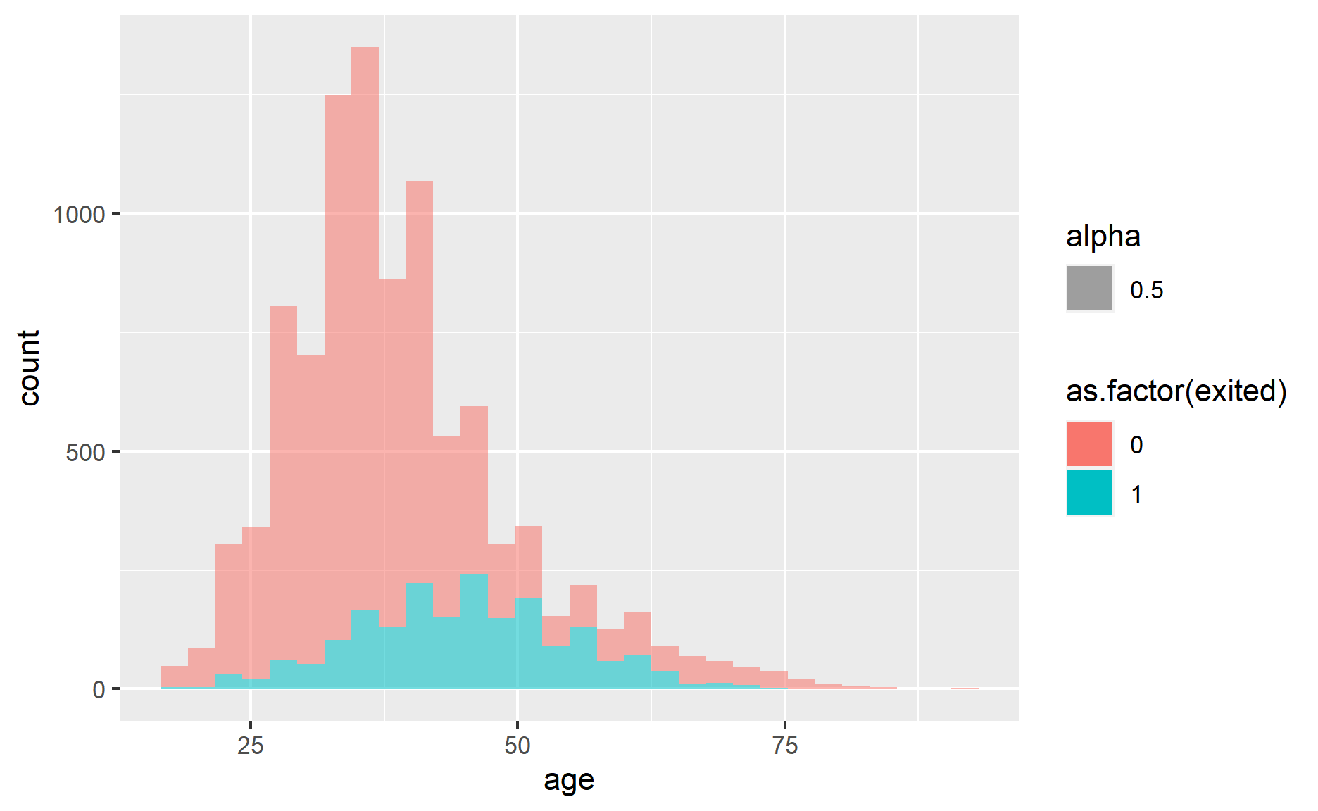
This comparison is useful for demonstration, but it should be interpreted carefully. Since the male and female models are fitted separately, the curves are not simply showing the isolated effect of gender from a single model. Another approach would be to create specific covariate profiles and use survfit(cox_model, newdata = ...) to compare predicted survival curves while holding other variables fixed.
Visualise the Cox proportional hazards results
Next, I will visualise the fitted model results with a forest plot of the hazard ratios.
plot_hazard_ratios <- function(model) {
  model_summary <- summary(model)

  hazard_ratios <-
    as_tibble(model_summary$conf.int, rownames = "term") %>%
    select(term,
           hazard_ratio = `exp(coef)`,
           lower_ci = `lower .95`,
           upper_ci = `upper .95`) %>%
    left_join(
      as_tibble(model_summary$coefficients, rownames = "term") %>%
        transmute(term, p_value = `Pr(>|z|)`),
      by = "term"
    ) %>%
    mutate(term = fct_reorder(term, hazard_ratio))

  ggplot(hazard_ratios,
         aes(x = hazard_ratio,
             y = term,
             xmin = lower_ci,
             xmax = upper_ci,
             color = p_value < 0.05)) +
    geom_vline(xintercept = 1, linetype = "dashed", color = "grey50") +
    geom_pointrange() +
    scale_x_log10() +
    scale_color_manual(values = c("grey50", "#0072B2"), guide = "none") +
    labs(x = "Hazard ratio (log scale)",
         y = NULL)
}

plot_hazard_ratios(cox_model)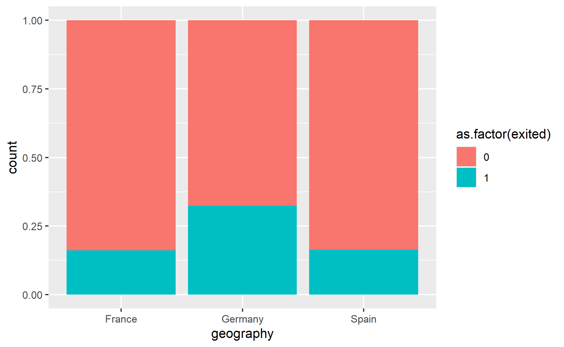
This graph contains the variables used in the Cox model and the categories within categorical variables.
On the right side of the graph, we have the hazard ratio, the confidence interval, and the p-value for each variable.
As discussed earlier, a higher hazard ratio indicates a higher hazard of churn, while a lower hazard ratio indicates a lower hazard of churn, conditional on the other variables in the model.
For example, the rendered model output shows that genderMale has a hazard ratio of approximately 0.68. This suggests that, holding the other variables constant, male customers have about 32% lower churn hazard than the reference group, which is female customers.
For a numerical variable, the hazard ratio can be interpreted as the change in hazard for every one-unit increase in that variable. For example, the rendered model output shows an age hazard ratio of approximately 1.05. This means a one-year increase in age is associated with about a 5% higher churn hazard, holding the other variables constant.
Based on the Cox model result, several patterns stand out:
- Churn hazard appears to increase with age.
ggplot(df, aes(x = age, fill = as.factor(exited), alpha = 0.5)) +
  geom_histogram()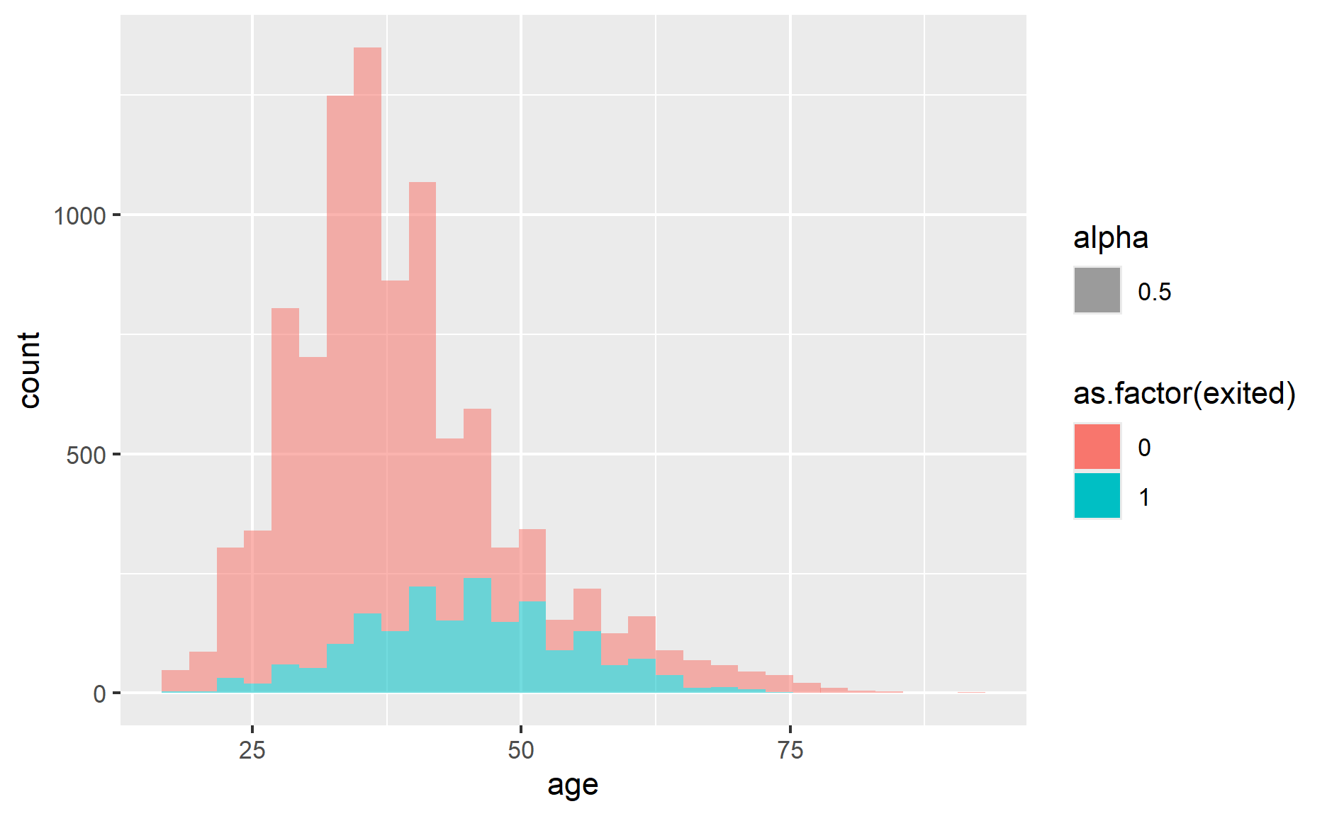
Churn hazard differs by active membership status. Customers tagged as inactive have a higher churn risk, so the company may want to design campaigns to re-engage inactive customers.
Customers from Germany are more likely to churn compared with customers from France, while Spain does not appear materially different from France in the fitted model.
This is consistent with what we observe in the dataset.
It is worth investigating why Germany has a higher churn rate.
For example, German customers may differ by product mix, acquisition channel, pricing, service experience, or another characteristic not captured in the dataset.
This additional analysis would help determine whether geography itself is important, or whether it is acting as a proxy for another customer characteristic.
ggplot(df, aes(x = geography, fill = as.factor(exited))) +
  geom_bar(position = "fill")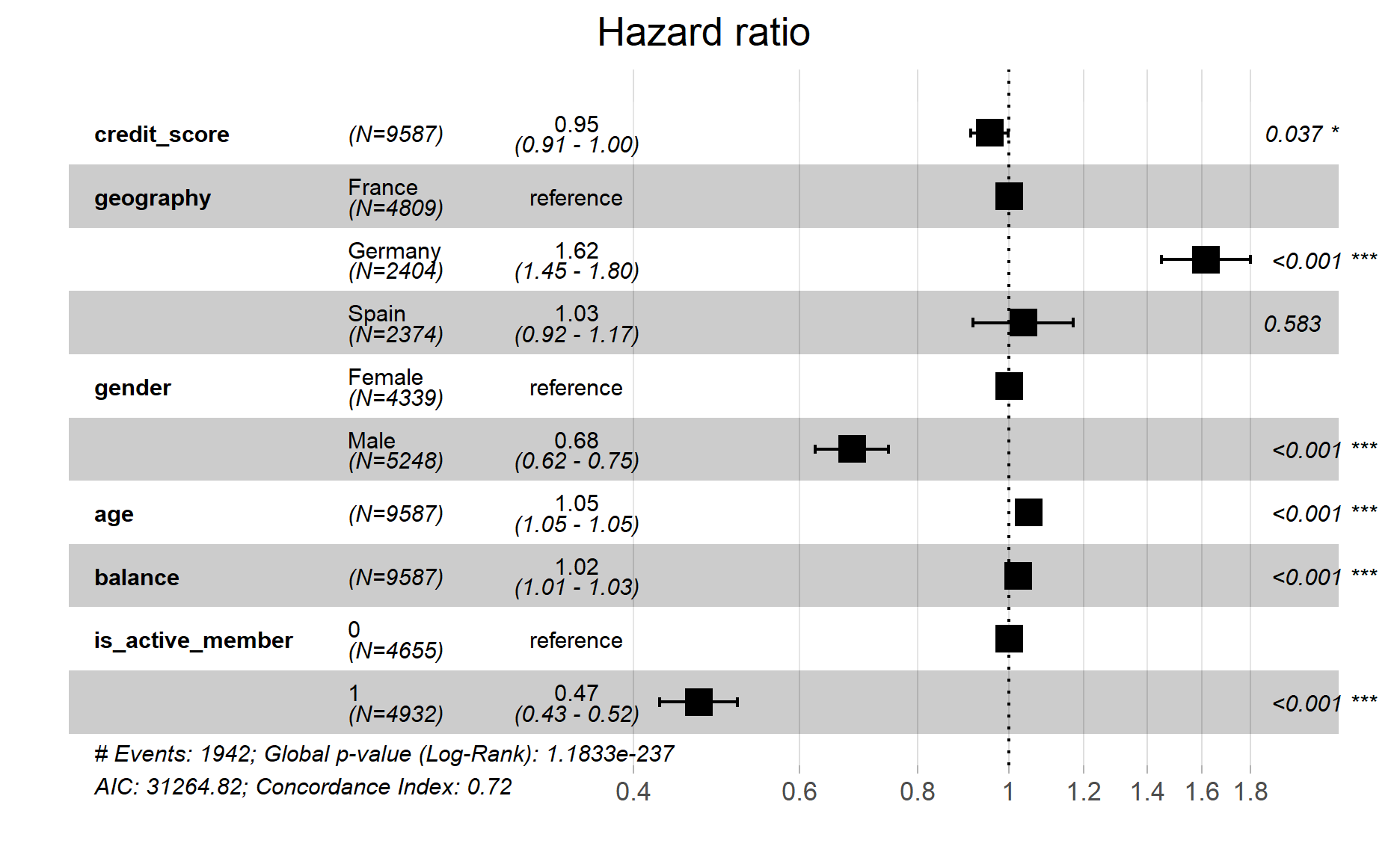
Feature selection
We can take one step further by performing feature selection on the variables used in the Cox proportional hazards model.
Here, I will use the step function from the stats package to perform stepwise feature selection.
Note that this method uses AIC to select the model.
I will also indicate that the direction should be "both", meaning the model can include or exclude variables at each step.
Start:  AIC=31267.66
Surv(tenure, exited) ~ credit_score + geography + gender + age +
    balance + num_of_products + has_cr_card + is_active_member +
    estimated_salary

                   Df   AIC
- estimated_salary  1 31266
- has_cr_card       1 31267
- num_of_products   1 31267
<none>                31268
- credit_score      1 31270
- balance           1 31286
- gender            1 31336
- geography         2 31348
- age               1 31881

Step:  AIC=31265.75
Surv(tenure, exited) ~ credit_score + geography + gender + age +
    balance + num_of_products + has_cr_card + is_active_member

                   Df   AIC
- has_cr_card       1 31265
- num_of_products   1 31265
<none>                31266
+ estimated_salary  1 31268
- credit_score      1 31268
- balance           1 31284
- gender            1 31334
- geography         2 31347
- age               1 31879

Step:  AIC=31265.16
Surv(tenure, exited) ~ credit_score + geography + gender + age +
    balance + num_of_products + is_active_member

                   Df   AIC
- num_of_products   1 31265
<none>                31265
+ has_cr_card       1 31266
+ estimated_salary  1 31267
- credit_score      1 31268
- balance           1 31284
- gender            1 31334
- geography         2 31345
- age               1 31880

Step:  AIC=31264.82
Surv(tenure, exited) ~ credit_score + geography + gender + age +
    balance + is_active_member

                   Df   AIC
<none>                31265
+ num_of_products   1 31265
+ has_cr_card       1 31265
+ estimated_salary  1 31267
- credit_score      1 31267
- balance           1 31289
- gender            1 31333
- geography         2 31344
- age               1 31883
Call:
coxph(formula = Surv(tenure, exited) ~ credit_score + geography +
gender + age + balance + is_active_member, data = df, x = TRUE,
y = TRUE)
coef exp(coef) se(coef) z p
credit_score -0.048060 0.953076 0.023066 -2.084 0.0372
geographyGermany 0.479384 1.615078 0.055375 8.657 < 2e-16
geographySpain 0.034141 1.034731 0.062170 0.549 0.5829
genderMale -0.383472 0.681491 0.045820 -8.369 < 2e-16
age 0.048282 1.049466 0.001813 26.631 < 2e-16
balance 0.022047 1.022292 0.004329 5.093 3.53e-07
is_active_member1 -0.757448 0.468862 0.048702 -15.553 < 2e-16
Likelihood ratio test=1120 on 7 df, p=< 2.2e-16
n= 9587, number of events= 1942 From the result, the following variables are dropped during feature selection:
num_of_products
has_cr_card
estimated_salary
With this, I will rebuild the Cox proportional hazards model with fewer variables.
cox_model_sub <-
  coxph(Surv(tenure, exited) ~ credit_score + geography + gender + age + balance + is_active_member,
        data = df,
        x = TRUE,
        y = TRUE)

plot_hazard_ratios(cox_model_sub)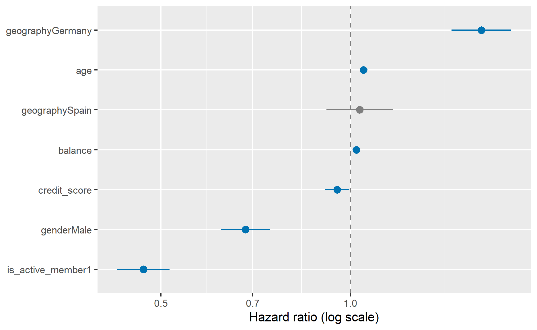
Next, I will extract the concordance index of the new model.
cox_model_sub$concordance["concordance"]concordance
0.7200558 The new model requires fewer variables, while the concordance index only drops slightly.
The concordance index dropped by 0.06%.
That said, stepwise selection should be used carefully. It can produce unstable variable selections, especially when predictors are correlated. A more complete modelling workflow would also consider:
domain knowledge and whether each variable is available at prediction time
train/test or cross-validation performance
proportional hazards diagnostics
non-linear effects, such as using splines for age or balance
interactions, such as whether age behaves differently by geography or active membership status
calibration, not only ranking performance
business usefulness, such as whether the model can support targeted churn-prevention actions
Conclusion
The Cox proportional hazards model is a useful tool when we want to understand how different variables are associated with the timing of an event. Its main strength is that it can model multiple covariates while leaving the baseline hazard unspecified.
In this example, the model suggests that churn hazard is associated with age, geography, gender, balance, and active membership status. The model also achieves an in-sample C-index of around 0.72, suggesting reasonable ranking ability.
However, a complete survival analysis should go beyond fitting the model. We should check the proportional hazards assumption, validate performance on unseen data, consider calibration, and confirm that the time and censoring definitions are appropriate for the business problem.
Thanks for reading the post until the end.
Feel free to contact me through email or LinkedIn if you have any suggestions on future topics to share.
Refer to this link for the blog disclaimer.
Till next time, happy learning!

Photo by Helena Lopes