
Photo by sydney Rae on Unsplash
When we analyse data, we often use a sample to learn something about a larger population. For example, we may use penguins observed in a research dataset to estimate the average body mass of a penguin species.
A sample mean is useful, but it is incomplete on its own. If we collect a different sample, we will probably get a slightly different mean. A confidence interval helps us express this uncertainty.
What is a confidence interval?
A confidence interval is a range of plausible values for an unknown population parameter.
For example, suppose we want to estimate the true mean body mass of Adelie penguins. We can calculate the mean body mass from the sample, but the sample mean is only an estimate. A confidence interval adds a lower and upper bound around that estimate.
In simple terms, a confidence interval answers this question:
Based on the data we observed, what range of values is reasonable for the population quantity we are trying to estimate?
The most common confidence level is 95%. A 95% confidence interval is usually written as:
\[ \text{estimate} \pm \text{margin of error} \]
For a mean, the confidence interval is commonly computed as:
\[ \bar{x} \pm t^* \times \frac{s}{\sqrt{n}} \]
where:
- \(\bar{x}\) is the sample mean
- \(t^*\) is the critical value from the t-distribution
- \(s\) is the sample standard deviation
- \(n\) is the sample size
- \(\frac{s}{\sqrt{n}}\) is the standard error
When should we use a confidence interval?
Confidence intervals are useful when we want to estimate a population parameter and communicate the uncertainty around that estimate.
We commonly use confidence intervals when estimating:
- a population mean, such as average body mass
- a population proportion, such as the proportion of observations in a category
- the difference between two means
- the difference between two proportions
- regression coefficients
- model predictions
Confidence intervals are especially helpful when we do not want to rely only on a point estimate. Instead of saying “the average is 3700 grams”, we can say “the average is estimated to be 3700 grams, with a 95% confidence interval from 3550 to 3850 grams”. The second statement is more informative because it shows the precision of the estimate.
As a rule of thumb, use a confidence interval when:
- the goal is estimation, not just prediction
- the data are a sample from a broader population or process
- uncertainty matters for interpretation or decision-making
- you want to compare groups and understand whether differences are precise or uncertain
How do we interpret a confidence interval?
The interpretation of a confidence interval is subtle. A 95% confidence interval does not mean that there is a 95% probability that the true population value is inside the interval after the interval has been calculated. In frequentist statistics, the population value is treated as fixed, while the interval varies from sample to sample.
A better interpretation is:
If we repeatedly collected samples using the same method and calculated a 95% confidence interval from each sample, about 95% of those intervals would contain the true population parameter.
For a single interval, we can say that the interval gives a range of plausible values for the population parameter, given the data and assumptions.
The width of a confidence interval is also important. A narrow interval suggests a more precise estimate. A wide interval suggests more uncertainty.
Confidence intervals become narrower when:
- the sample size is larger
- the data are less variable
- the confidence level is lower
Confidence intervals become wider when:
- the sample size is smaller
- the data are more variable
- the confidence level is higher
Demonstration in R
In this demonstration, I will use the penguins dataset from the palmerpenguins package.
The dataset contains measurements for three penguin species: Adelie, Chinstrap, and Gentoo.
We will compute a 95% confidence interval for the mean body mass of Adelie penguins.
Load and inspect the data
data("penguins")

penguins %>%
  glimpse()
Rows: 344
Columns: 8
$ species <fct> Adelie, Adelie, Adelie, Adelie, Adelie, Ad…
$ island <fct> Torgersen, Torgersen, Torgersen, Torgersen…
$ bill_length_mm <dbl> 39.1, 39.5, 40.3, NA, 36.7, 39.3, 38.9, 39…
$ bill_depth_mm <dbl> 18.7, 17.4, 18.0, NA, 19.3, 20.6, 17.8, 19…
$ flipper_length_mm <int> 181, 186, 195, NA, 193, 190, 181, 195, 193…
$ body_mass_g <int> 3750, 3800, 3250, NA, 3450, 3650, 3625, 46…
$ sex <fct> male, female, female, NA, female, male, fe…
$ year <int> 2007, 2007, 2007, 2007, 2007, 2007, 2007, …The variable body_mass_g gives the body mass of each penguin in grams.
Before computing the confidence interval, I will filter the data to one species and remove missing values.
adelie <- penguins %>%
  filter(species == "Adelie") %>%
  drop_na(body_mass_g)

adelie %>%
  summarise(
    n = n(),
    mean_body_mass = mean(body_mass_g),
    sd_body_mass = sd(body_mass_g)
  ) %>%
kable(digits = 2)| n | mean_body_mass | sd_body_mass |
|---|---|---|
| 151 | 3700.66 | 458.57 |
Compute the confidence interval manually
To compute the confidence interval manually, we need the sample mean, sample standard deviation, sample size, standard error, and the critical value from the t-distribution.
adelie_summary <- adelie %>%
  summarise(
    n = n(),
    mean_body_mass = mean(body_mass_g),
    sd_body_mass = sd(body_mass_g),
    standard_error = sd_body_mass / sqrt(n),
    t_critical = qt(0.975, df = n - 1),
    margin_of_error = t_critical * standard_error,
    lower_ci = mean_body_mass - margin_of_error,
    upper_ci = mean_body_mass + margin_of_error
  )

adelie_summary %>%
kable(digits = 2)| n | mean_body_mass | sd_body_mass | standard_error | t_critical | margin_of_error | lower_ci | upper_ci |
|---|---|---|---|---|---|---|---|
| 151 | 3700.66 | 458.57 | 37.32 | 1.98 | 73.74 | 3626.93 | 3774.4 |
The expression qt(0.975, df = n - 1) gives the critical value for a two-sided 95% confidence interval.
We use 0.975 because 2.5% of the probability is in the lower tail and 2.5% is in the upper tail.
Compute the confidence interval using t.test()
R can also compute the confidence interval directly using t.test().
Although t.test() is often introduced as a hypothesis testing function, it also returns a confidence interval for the mean.
adelie_t_test <- t.test(adelie$body_mass_g, conf.level = 0.95)

adelie_t_test
    One Sample t-test

data:  adelie$body_mass_g
t = 99.167, df = 150, p-value < 2.2e-16
alternative hypothesis: true mean is not equal to 0
95 percent confidence interval:
 3626.926 3774.398
sample estimates:
mean of x
 3700.662
We can extract the confidence interval from the result:
adelie_t_test$conf.int[1] 3626.926 3774.398
attr(,"conf.level")
[1] 0.95The result should match the manual calculation, apart from small rounding differences.
Confidence intervals by species
We can also compute confidence intervals for each penguin species. This is useful when we want to compare group means and understand the uncertainty around each estimate.
species_ci <- penguins %>%
  drop_na(species, body_mass_g) %>%
  group_by(species) %>%
  summarise(
    n = n(),
    mean_body_mass = mean(body_mass_g),
    sd_body_mass = sd(body_mass_g),
    standard_error = sd_body_mass / sqrt(n),
    t_critical = qt(0.975, df = n - 1),
    lower_ci = mean_body_mass - t_critical * standard_error,
    upper_ci = mean_body_mass + t_critical * standard_error,
    .groups = "drop"
  )

species_ci %>%
kable(digits = 2)| species | n | mean_body_mass | sd_body_mass | standard_error | t_critical | lower_ci | upper_ci |
|---|---|---|---|---|---|---|---|
| Adelie | 151 | 3700.66 | 458.57 | 37.32 | 1.98 | 3626.93 | 3774.40 |
| Chinstrap | 68 | 3733.09 | 384.34 | 46.61 | 2.00 | 3640.06 | 3826.12 |
| Gentoo | 123 | 5076.02 | 504.12 | 45.45 | 1.98 | 4986.03 | 5166.00 |
We can visualise the confidence intervals using an error bar plot.
species_ci %>%
  ggplot(aes(x = species, y = mean_body_mass, colour = species)) +
  geom_point(size = 3) +
  geom_errorbar(
    aes(ymin = lower_ci, ymax = upper_ci),
    width = 0.15,
    linewidth = 0.8
  ) +
  labs(
    x = "Species",
    y = "Mean body mass (g)",
    title = "95% confidence intervals for mean penguin body mass"
  ) +
  theme_minimal() +
  theme(legend.position = "none")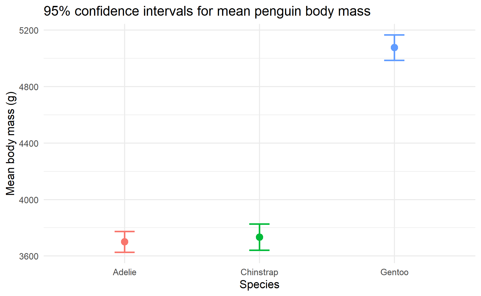
Each point shows the sample mean body mass for a species. Each vertical line shows the 95% confidence interval around that mean.
Common misunderstandings
There are a few common mistakes when interpreting confidence intervals.
First, a 95% confidence interval does not mean that 95% of the data fall inside the interval. The interval is about uncertainty in the estimated population parameter, not the spread of individual observations.
Second, a 95% confidence interval does not mean there is a 95% probability that the specific calculated interval contains the true value. The 95% refers to the long-run success rate of the method used to create the interval.
Third, overlapping confidence intervals do not automatically mean that two groups are not meaningfully different. Confidence intervals are useful for comparison, but formal comparisons usually require estimating the difference between groups directly.
Conclusion
A confidence interval is a practical way to describe uncertainty around an estimate. Instead of reporting only one number, we report a range of plausible values.
In this post, we covered:
- what a confidence interval is
- when to use a confidence interval
- how to interpret a confidence interval
- how to compute a confidence interval manually in R
- how to compute a confidence interval using
t.test() - how to visualise confidence intervals across groups using the
penguinsdataset
Confidence intervals are one of the most useful tools in statistics because they encourage us to think beyond point estimates. They remind us that estimates from data are useful, but they are also uncertain.

Photo by Towfiqu barbhuiya on Unsplash
Thanks for reading the post until the end.
Feel free to contact me through email or LinkedIn if you have any suggestions on future topics to share.
Refer to this link for the blog disclaimer.
Till next time, happy learning!